Contact
Feel free to reach out through my social media.
Leveraging Natural Language Processing to understand market sentiment and financial trends.
Marco A. García - 12/01/2025
You can find this project in the GitHub repository.

In this project, we analyze a dataset of financial news to gain insights into the sentiment and trends present in financial media. This involves several key steps, including:
Our goal is to uncover patterns in financial sentiment and understand how news impacts financial markets.
The dataset contains fields like:
Let’s dive into the analysis!
In this project, we will use the following Python packages to perform various text analysis and visualization tasks:
These packages provide a comprehensive set of tools to handle the entire pipeline of text analysis, from data preparation to visualization.
import pandas as pd

import nltk
from nltk import word_tokenize
nltk.download('punkt_tab')

from nltk.corpus import stopwords
nltk.download("stopwords")

from nltk.stem.porter import PorterStemmer

import matplotlib.pyplot as plt

from nltk.sentiment.vader import SentimentIntensityAnalyzer
nltk.download("vader_lexicon")

from wordcloud import WordCloud
[nltk_data] Downloading package punkt_tab to /root/nltk_data...
[nltk_data] Unzipping tokenizers/punkt_tab.zip.
[nltk_data] Downloading package stopwords to /root/nltk_data...
[nltk_data] Unzipping corpora/stopwords.zip.
[nltk_data] Downloading package vader_lexicon to /root/nltk_data...The first step in our analysis is to prepare the dataset and create a corpus. This involves loading the data, cleaning it, and formatting it into a structure that can be analyzed effectively.
df = pd.read_csv("financial-news.csv")
df.shape
(28276, 8)As we can see, we have a total of 28,276 registers and 8 features.
After reviewing the dataset, I will preserve only the “text” feature for the corpus. This is because it is the only feature that contains meaningful text data relevant for our analysis. Other features, while informative, are not directly related to the sentiment and content of the financial news.
corpus = df["text"]After creating the corpus, it is essential to ensure that it does not
contain any missing values (NaN). Missing values can interfere with
text processing and lead to errors in subsequent analysis.
corpus[corpus.isna()]With a clean, non-NaN corpus, the next step is to check for duplicate entries. Duplicate values can skew the analysis by over-representing certain text entries, so it is important to identify and handle them appropriately.
corpus[corpus.duplicated()]2584 rows × 1 columns
After verifying for duplicates, we found that the corpus contains 2,584 duplicated values. To ensure the quality and diversity of the data, we will remove these duplicates.
corpus = corpus.drop_duplicates(keep="first")
corpus.shape(25692,)After removing duplicated values, we reduced the total number of entries in the corpus from 28,276 to 25,692. This remains a substantial amount of data for meaningful analysis.
Analyzing the frequency of text lengths in the corpus provides insights into the distribution of the data and helps identify patterns in the length of financial news articles or posts.
Before adding new features, it is essential to confirm the type of the
corpus object to ensure compatibility with the operations we want to
perform.
print(type(corpus))<class 'pandas.core.series.Series'>Since the corpus is currently a pandas.Series, we need to convert it
into a pandas.DataFrame to add additional columns. We will use the
apply method to calculate the length of each text entry and include it
as a new column called doc_len.
corpus = pd.DataFrame({
    "text": corpus,
    "doc_len": corpus.apply(lambda x: len(x))
})

corpus.head(3)
25692 rows × 2 columns
With the doc_len column added to the corpus DataFrame, we can now
explore the minimum and maximum lengths of the texts. This helps us
understand the range of text lengths and identify outliers or unusual
entries.
print("Min:", corpus["doc_len"].min())
print("Max:", corpus["doc_len"].max())
Min: 2
Max: 71521Identifying texts with lengths below 20 characters helps us examine potentially anomalous or overly concise entries. These texts might not carry meaningful information and may require additional consideration during analysis.
corpus[corpus["doc_len"] < 20]129 rows × 2 columns
After reviewing the corpus, we found that 129 entries with lengths below 20 characters lack meaningful information. To maintain the quality of the dataset, we will filter out these entries.
corpus = corpus[corpus["doc_len"] > 20]
corpus.shape
(25557, 2)Tokenization is the process of transforming text into meaningful lexical tokens. This step is essential because:
Efficient Processing: Smaller units of text are easier to analyze and process.
Numeric Representations: Tokens can be transformed into numerical representations for machine learning tasks.
Simplifies Text Modeling: Tokenized text is foundational for many natural language processing (NLP) tasks.
To perform tokenization, we will use NLTK (Natural Language Toolkit), a Python package designed for various NLP tasks, including tokenization.
corpus["tokens"] = corpus["text"].apply(lambda x: word_tokenize(x.lower()))corpus.head(3)25557 rows × 3 columns
Now that we have the tokenized representation of each text, we can calculate the number of tokens for each entry. This information will help us understand the token distribution across the corpus and identify any anomalies before proceeding with stopword removal.
corpus["number_tokens"] = corpus["tokens"].apply(lambda x: len(x))corpus.head(3)25557 rows × 4 columns
Stopwords are common words (e.g., “the”, “and”, “is”) that do not contribute meaningful information to the analysis. Removing stopwords reduces noise in the dataset and improves the quality of insights derived from the text.
To streamline the process of removing stopwords, we will create a custom function that:
stopwords.words method from nltk.This function will then be applied to each row of the corpus.
def remove_stopwords(tokens, lang="english"):
  stopwords_list = stopwords.words(lang)
return [token for token in tokens if token not in stopwords_list]corpus["tokens"] = corpus["tokens"].apply(lambda x: remove_stopwords(x))
corpus["number_tokens"] = corpus["tokens"].apply(lambda x: len(x))corpus.head(3)25557 rows × 4 columns
Stemming is the process of reducing words to their base or root form. For example, “running” becomes “run” and “studies” becomes “studi”. Stemming helps normalize the text by grouping words with similar meanings under a common root.
porter_stemmer = PorterStemmer()

def stem_tokens(tokens):
return [porter_stemmer.stem(token) for token in tokens]corpus["tokens"] = corpus["tokens"].apply(lambda x: stem_tokens(x))
corpus.head(3)25557 rows × 4 columns
With the text data fully processed, we can now explore the corpus using various visualizations. These visualizations help uncover patterns, trends, and key insights in the dataset.
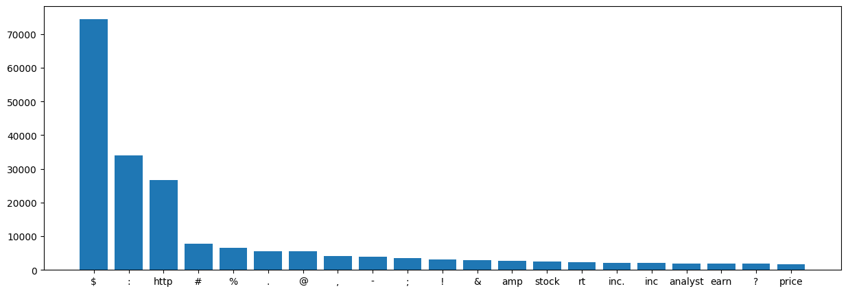
To understand the most frequently occurring words in the corpus, we will analyze the 20 most repeated tokens. This helps identify key themes and topics in the dataset.
corpus_tokens = list(corpus["tokens"])tokens_count = {}
for document_tokens in corpus_tokens:
for token in document_tokens:
if token in tokens_count:
tokens_count[token] = tokens_count[token] + 1
else:
tokens_count[token] = 1
ordered_tokens_count = sorted(tokens_count.items(), key=lambda x: x[1], reverse=True)def plot_tokens_frequency(tokens):
fig, ax = plt.subplots(figsize=(15, 5))
labels = [item[0] for item in tokens]
counts = [item[1] for item in tokens]
plt.bar(labels, counts)plot_tokens_frequency(ordered_tokens_count[0:21])
Based on the bar chart:
Dollar Sign ($):
http:
Punctuation and Special Characters:
:, #, %, @, !, and others are common. They
reflect the nature of tweets or short-form financial news, where
special characters are often used.#, @) indicate hashtags and
mentions, which may hold valuable context in social media-based
financial analysis.Financial Lexical Tokens:
stock, price, earn, and analyst are highly
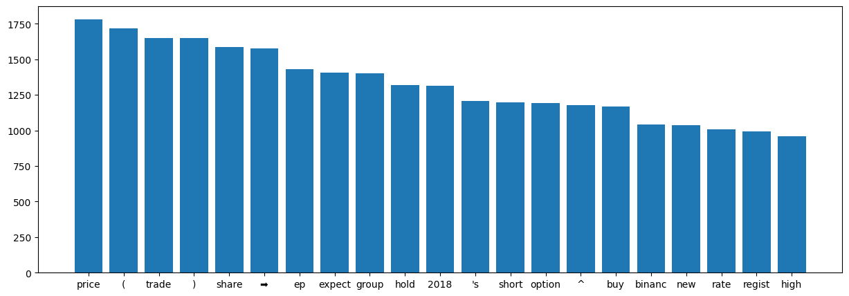
frequent, highlighting the focus on financial discussions.To gain a deeper understanding of the corpus, we will analyze the next 20 most repeated tokens, excluding the first 20 that we already examined. This will help uncover additional patterns and frequent terms that may not have been immediately apparent.
plot_tokens_frequency(ordered_tokens_count[20:41])
From the new chart, we observe tokens such as “hold”, “buy”, and “high”, which suggest an inclination toward upward financial trends. In contrast, “short” could represent downward trends or a bearish sentiment. To validate this hypothesis, we will apply sentiment analysis to the corpus.
Sentiment analysis helps us determine the emotional tone or polarity of the text data. This step is particularly useful for financial datasets to understand whether the overall sentiment is positive, negative, or neutral. It also helps uncover sentiment trends associated with specific tokens like “buy”, “hold”, or “short”.
To enhance the analysis, we will classify each text entry in the corpus as Positive, Negative, or Neutral based on its sentiment polarity score. For this, we will define a function that uses the VADER sentiment analyzer to calculate the sentiment score and assign a label accordingly.
sentiment_analyzer = SentimentIntensityAnalyzer()

def sentiment_classification(text):
  result = sentiment_analyzer.polarity_scores(text)["compound"]
  if result >= 0.5:
    return "Positive"
  elif result <= -0.5:
    return "Negative"
  else:
return "Neutral"corpus["sentiment"] = corpus["tokens"].apply(lambda x: sentiment_classification(" ".join(x)))corpus.head(3)25557 rows × 5 columns
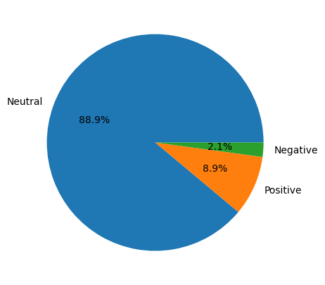
With the sentiment classification added to the corpus, we can now create a visualization to see the distribution of sentiments (Positive, Negative, Neutral) across the dataset. This helps us understand the overall emotional tone of the financial news corpus.
fig, ax = plt.subplots(figsize=(15, 5))

sentiments = corpus["sentiment"].value_counts()

labels = sentiments.index
sizes = sentiments.values

ax.pie(sizes, labels=labels, autopct="%1.1f%%")

plt.show()
The pie chart reveals that the most predominant sentiment in the dataset is Neutral, followed by Positive, with Negative being the least frequent. This distribution offers significant insights:
Neutral Sentiment (88.9%):
Positive Sentiment (8.9%):
Negative Sentiment (2.1%):
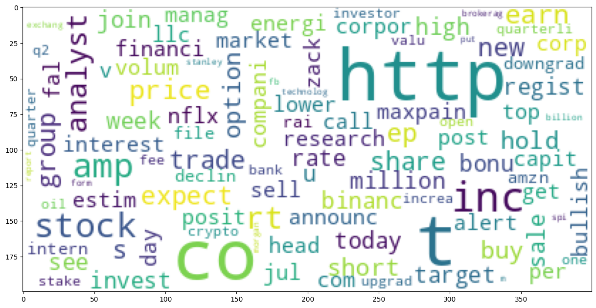
A Word Cloud is a visually engaging way to represent the frequency of words in a text corpus. Words that appear more frequently are displayed in larger fonts, allowing us to quickly identify dominant themes or topics.
def display_word_cloud(corpus, stopwords=[], color="white"):
  stopwords = set(stopwords)
  wordcloud = WordCloud(
      background_color=color,
      stopwords=stopwords,
      max_words=100,
      max_font_size=50,
      random_state=1,
      collocations=False
  )

  wordcloud = wordcloud.generate(str(corpus))

  fig, ax = plt.subplots(figsize=(15, 15))
  plt.imshow(wordcloud)
  plt.axis("on")
  plt.show()
corpus_string = " ".join(token for vector_tokens in corpus["tokens"] for token in vector_tokens)display_word_cloud(corpus_string)
The Word Cloud provides valuable insights, but it also contains noise, such as tokens like “http” and other terms that may not be relevant to our analysis. To refine the visualization, we can pass a custom list of stopwords to exclude these terms.
display_word_cloud(corpus_string, ["http", "co", "com", "t", "inc", "s", "u"])
The refined Word Cloud highlights a cleaner representation of the most frequently used words in the financial news corpus. By removing irrelevant tokens like “http”, “com”, and others, the visualization provides more meaningful insights.
Key Observations:
Dominant Words:
Emerging Themes:
Directional Sentiments:
The analysis of the financial news dataset provided valuable insights into the sentiment and thematic composition of the data. Here are the main conclusions and potential actions one can take based on these findings:
Predominantly Neutral Sentiment:
Presence of Positive and Negative Sentiment:
Frequent Financial Lexicon:
Market Strategy Development:
Neutral Sentiment: Companies and investors can view neutral sentiment as a signal of market steadiness, suitable for long-term strategic decisions.
Positive Sentiment: A rise in positive sentiment (e.g., “buy”, “high”, “earn”) can signal opportunities for investment or market entry.
Negative Sentiment: Negative sentiment (e.g., “short”, “sell”) can be an early warning for risk management, encouraging diversification or short-term hedging strategies.
Trend Monitoring:
Content Creation and Communication:
Data-Driven Decision Making:
This analysis demonstrates how businesses, investors, and market participants can leverage sentiment analysis and financial lexicon insights to make informed decisions. Whether it’s identifying growth opportunities, mitigating risks, or understanding market trends, the processed data provides actionable intelligence to stay competitive in dynamic financial markets.
Feel free to reach out through my social media.