You can find this project in the GitHub repository.

Employee Attrition Prediction: A Comparative Analysis of Machine Learning Models

In this article, we will explore the process of predicting employee attrition using various machine learning models. We’ll walk through data loading, preprocessing, model selection, hyperparameter tuning, and ultimately, model comparison to determine the best performer. We’ll be using Python with the scikit-learn (sklearn) library for this task.

1. Library Inclusion

First, let’s import the necessary libraries.

import pandas as pd
import numpy as np

import matplotlib.pyplot as plt

from sklearn.model_selection import train_test_split
from sklearn.preprocessing import StandardScaler
from sklearn.model_selection import cross_validate
from sklearn.model_selection import RandomizedSearchCV
from sklearn.model_selection import GridSearchCV

from sklearn.ensemble import RandomForestClassifier
from sklearn.linear_model import LogisticRegression
from sklearn.naive_bayes import GaussianNB
from sklearn.svm import SVC

from sklearn.metrics import ConfusionMatrixDisplay
from sklearn.metrics import classification_report
from sklearn.metrics import RocCurveDisplay

import warnings
warnings.filterwarnings("ignore")

This code imports essential libraries:

• pandas for data manipulation.
• numpy for numerical operations.
• matplotlib.pyplot for data visualization.
• sklearn modules for model building, preprocessing, and evaluation.
• warnings to suppress warning messages for cleaner output.

2. Data Acquisition

Now, let’s load the dataset from a CSV file named “Employee_Attrition.csv”.

data = pd.read_csv("Employee_Attrition.csv")

This line reads the CSV file into a pandas DataFrame called data.

3. Data Analysis

Let’s take a peek at the dataset’s structure and content.

data.info()

This code displays information about the DataFrame, including column names, data types, and the number of non-null values.

data["Attrition"].value_counts()

This code snippet counts the occurrences of each unique value in the “Attrition” column, providing a sense of the class distribution. In our case, it shows how many employees stayed (No) and how many left (Yes).

Class Imbalance Note: The initial data exploration reveals a significant class imbalance, with far more employees who did not leave (“No”) than those who did (“Yes”). This imbalance can bias models toward the majority class. To address this, we will utilize the class_weight parameter in our models where available. This parameter adjusts the weight given to each class during training, penalizing misclassifications of the minority class more heavily.

4. Variable Elimination

Some variables are deemed irrelevant for prediction and are removed to simplify the model and improve performance.

data.nunique()

This outputs the number of unique values in each column. This help us to identify features that might not be useful for the prediction, for example a column with only one value.

relevant_data = data.drop(columns=["EmployeeCount", "EmployeeNumber", "Over18", "StandardHours"])
relevant_data.columns

Here, we drop columns “EmployeeCount,” “EmployeeNumber,” “Over18,” and “StandardHours” because they contain little to no variance or are irrelevant to employee attrition.

5. Categorical Variable Transformation

Machine learning models typically require numerical input. Therefore, categorical variables need to be transformed into a numerical representation. Here, we use One-Hot Encoding.

numeric_data = relevant_data.copy()

for c in numeric_data.columns:
  if numeric_data[c].dtypes == "object":
    numeric_data = pd.get_dummies(numeric_data, columns=[c], dtype=int, drop_first=True)

numeric_data.dtypes

This code iterates through each column. If a column has an object data type (meaning it’s categorical), it’s transformed using pd.get_dummies. The drop_first=True argument prevents multicollinearity by dropping the first category of each feature.

6. Data Partitioning and Scaling

The data is split into training and testing sets to evaluate model performance on unseen data. Feature scaling is also applied to standardize the data.

X_df = numeric_data.drop(columns=["Attrition_Yes"])
y_df = numeric_data["Attrition_Yes"]

This code separates features (X) from the target variable (y). The target is “Attrition_Yes,” representing whether an employee left the company or not.

X_to_scale = X_df.to_numpy()
X_scaled = StandardScaler().fit_transform(X_to_scale)
X_df_scaled = pd.DataFrame(X_scaled, columns=X_df.columns)
X_df_scaled.head()

This scales the features using StandardScaler, which standardizes data by removing the mean and scaling to unit variance. This ensures that features with different scales do not unduly influence the models.

X = X_df_scaled.to_numpy()
y = y_df.to_numpy()

X_train, X_test, y_train, y_test = train_test_split(X, y, test_size=0.2)
X_train_with_validation, X_validation, y_train_with_validation, y_validation = train_test_split(X_train, y_train, test_size=0.25)

print("With validation:")
print("Train:", len(X_train_with_validation) * 100 / X.shape[0], "%")
print("Validation:", len(X_validation) * 100 / X.shape[0], "%")
print("Test:", len(X_test) * 100 / X.shape[0], "%")
print("\n")
print("Without validation")
print("Train:", len(X_train) * 100 / X.shape[0], "%")
print("Test:", len(X_test) * 100 / X.shape[0], "%")

This splits the data into training and testing sets (80/20 split). Additionally, the training data is further split into training and validation sets (60/20/20 split) in the case that we need to have an actual validation set that is no used by scikit-learn.

class_weight = {0: 1, 1: 5}

This defines the class_weight dictionary, which assigns a higher weight to the minority class (attrition = Yes) to address the class imbalance.

7. Model Building and Evaluation

Now, we’ll train and evaluate four different machine learning models: Random Forest, Logistic Regression, Gaussian Naive Bayes, and Support Vector Machine. For each model, we’ll first train it with default parameters, then perform hyperparameter tuning using grid search or randomized search.

7.1. Random Forest

rfc_default = RandomForestClassifier(class_weight=class_weight)
rfc_default.fit(X_train, y_train)
rfc_default_predictions = rfc_default.predict(X_test)
rfc_default_matrix = ConfusionMatrixDisplay.from_predictions(y_test, rfc_default_predictions)
rfc_default_classification_report = classification_report(y_test, rfc_default_predictions)
print(rfc_default_classification_report)

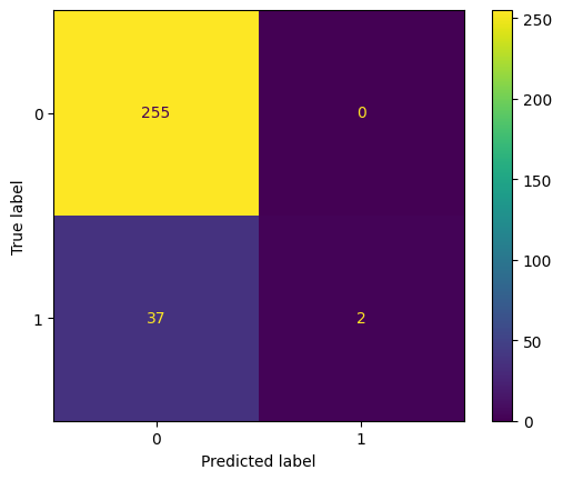
This code trains a Random Forest Classifier with default parameters and the defined class_weight. It then makes predictions on the test set, generates a confusion matrix, and prints the classification report (precision, recall, F1-score, support).

rfc_params = {'max_depth': [2, 3, 5, 7],
              'max_features': ['sqrt', 'log2', None],
              'n_estimators': [10, 30, 60, 100],
              }

rfc_grid = GridSearchCV(RandomForestClassifier(class_weight=class_weight), param_grid=rfc_params, return_train_score=True)

rfc_grid.fit(X_train, y_train)

print("Mejores hiperparámetros:", rfc_grid.best_params_)

This performs hyperparameter tuning using GridSearchCV. It defines a grid of hyperparameters to search over (rfc_params). GridSearchCV exhaustively searches all parameter combinations in the grid to find the best combination.

rfc_model = rfc_grid.best_estimator_
ConfusionMatrixDisplay.from_estimator(rfc_model, X_test, y_test)
rfc_model_classification_report = classification_report(y_test, rfc_model.predict(X_test))
print(rfc_model_classification_report)

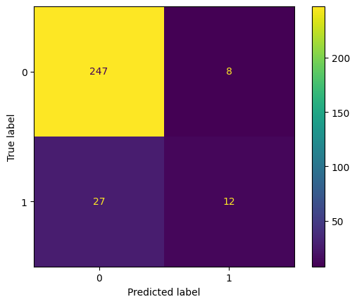
This code uses the best estimator found by GridSearchCV (rfc_model) to make predictions on the test set, generates a confusion matrix, and prints the classification report.

print("RFC default")
print(rfc_default_classification_report)
print()
print("RFC Grid Search")
print(rfc_model_classification_report)

This compares the classification reports of the default Random Forest model and the model trained with the best hyperparameters found by GridSearchCV.

rfc_final_model = rfc_model

We store the best Random Forest model as rfc_final_model.

7.2. Logistic Regression

lrc_default = LogisticRegression(class_weight=class_weight)
lrc_default.fit(X_train, y_train)
lrc_default_predictions = lrc_default.predict(X_test)
ConfusionMatrixDisplay.from_predictions(y_test, lrc_default_predictions)
lrc_default_classification_report = classification_report(y_test, lrc_default_predictions)
print(lrc_default_classification_report)

Similar to the Random Forest, this trains a Logistic Regression model with default parameters and class_weight, makes predictions, and prints the classification report.

lrc_params = {
    "C": np.logspace(-4, 4, 50),
    "solver": ["newton-cg", "lbfgs", "liblinear", "sag", "saga"],
}

lrc_rand = RandomizedSearchCV(
    LogisticRegression(class_weight=class_weight, random_state=42),
    n_iter=48,
    param_distributions=lrc_params,
    return_train_score=True
)

lrc_rand.fit(X_train, y_train)

print("Mejores hiperparámetros", lrc_rand.best_params_)

This performs hyperparameter tuning for Logistic Regression using RandomizedSearchCV. It defines a search space for C (regularization strength) and solver (optimization algorithm). RandomizedSearchCV randomly samples parameter combinations from the search space. n_iter controls the number of random combinations tested.

lrc_model = lrc_rand.best_estimator_
ConfusionMatrixDisplay.from_estimator(lrc_model, X_test, y_test)
lrc_model_classification_report = classification_report(y_test, lrc_model.predict(X_test))
print(lrc_model_classification_report)

This code evaluates the best Logistic Regression model found by RandomizedSearchCV.

print("LRC default")
print(lrc_default_classification_report)
print()
print("LRC Randomized Search")
print(lrc_model_classification_report)

This compares the default and tuned Logistic Regression models.

lrc_final_model = lrc_model

We store the best Logistic Regression model as lrc_final_model.

7.3. Gaussian Naive Bayes

gnbc_default = GaussianNB()
gnbc_default.fit(X_train, y_train)
gnbc_default_prediction = gnbc_default.predict(X_test)
ConfusionMatrixDisplay.from_predictions(y_test, gnbc_default_prediction)
print(classification_report(y_test, gnbc_default_prediction))

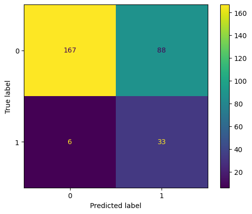
This trains a Gaussian Naive Bayes classifier with default parameters, makes predictions, and prints the classification report. Because Gaussian Naive Bayes has very few hyperparameters that meaningfully affect performance, hyperparameter tuning is skipped for this model.

gnbc_final_model = gnbc_default

We store the Gaussian Naive Bayes model as gnbc_final_model.

7.4. Support Vector Machine

svmc_default = SVC(class_weight=class_weight)
svmc_default.fit(X_train, y_train)
svmc_default_predictions = svmc_default.predict(X_test)
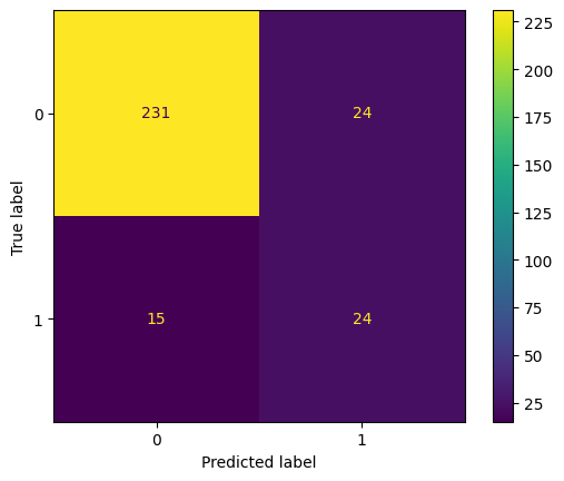
ConfusionMatrixDisplay.from_predictions(y_test, svmc_default_predictions)
svmc_default_classification_report = classification_report(y_test, svmc_default_predictions)
print(svmc_default_classification_report)

This trains a Support Vector Machine classifier with default parameters and class_weight, makes predictions, and prints the classification report.

svmc_params = {
    "C": [0.01, 0.1, 1, 10, 50],
    "kernel": ["linear", "poly", "rbf", "sigmoid"]
}

svmc_grid = GridSearchCV(SVC(class_weight=class_weight, random_state=42), param_grid=svmc_params, return_train_score=True)

svmc_grid.fit(X_train, y_train)

print("Mejores hiperparámetros", lrc_rand.best_params_)

This performs hyperparameter tuning for the SVM classifier using GridSearchCV. It searches over different values of C (regularization parameter) and kernel (kernel type). Note the random_state=42 to ensure reproducible results.

svmc_model = svmc_grid.best_estimator_

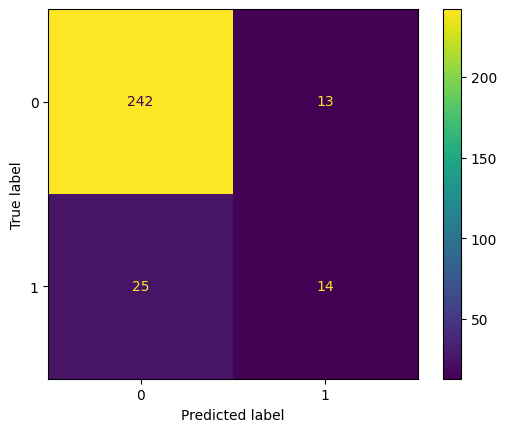
ConfusionMatrixDisplay.from_estimator(svmc_model, X_test, y_test)

svmc_model_classification_report = classification_report(y_test, svmc_model.predict(X_test))
print(svmc_model_classification_report)

This code evaluates the best SVM model found by GridSearchCV.

print("SVMC default")
print(svmc_default_classification_report)
print()
print("SVMC Grid Search")
print(svmc_model_classification_report)

This compares the default and tuned SVM models.

svmc_final_model = svmc_default

We store the best SVM model as svmc_final_model. In this case we kept the default values of the Support Vector Machine Classifier.

8. Model Comparison

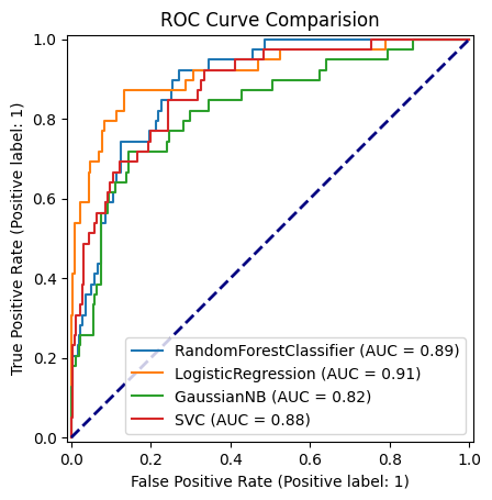
Finally, let’s compare the performance of the final models using ROC curves.

plt.figure()

lw=2

disp = RocCurveDisplay.from_estimator(rfc_final_model, X_test, y_test)
RocCurveDisplay.from_estimator(lrc_final_model, X_test, y_test, ax=disp.ax_)
RocCurveDisplay.from_estimator(gnbc_final_model, X_test, y_test, ax=disp.ax_)
RocCurveDisplay.from_estimator(svmc_final_model, X_test, y_test, ax=disp.ax_)

plt.plot([0, 1], [0, 1], color="navy", lw=lw, linestyle="--")
plt.title("ROC Curve Comparision")
plt.legend(loc="lower right")
plt.show()

This code generates ROC curves for all four final models on the test set. The ROC curve plots the true positive rate against the false positive rate at various threshold settings. The area under the ROC curve (AUC) is a common metric for evaluating the performance of classification models. A higher AUC indicates better performance.

9. Conclusion

The Logistic Regression model emerged as the best performer, achieving an impressive AUC of 0.91. This indicates its strong ability to distinguish between employees who are likely to leave and those who are likely to stay. While all models showed some ability to predict attrition, the Logistic Regression model provided the most reliable and accurate predictions based on the ROC AUC metric.

This article has demonstrated a complete machine learning workflow for predicting employee attrition, from data preprocessing and model selection to hyperparameter tuning and model comparison. By understanding these techniques, organizations can gain valuable insights into the factors driving employee turnover and develop targeted interventions to improve employee retention.